At my first introduction to measurement error, the word error gave me pause, and I silently wondered what good could possibly come from it. To most of us, an error usually means something is terribly wrong! It doesn’t help either that measurement error is somewhat misunderstood. Yet, without exception, every score in the educational setting has some degree of uncertainty—error. If we are to interpret scores correctly, we need to get comfortable with measurement error.

What Is Measurement Error?

Let’s begin with the traditional definition. You’ll probably be pleased that the bell-shaped curve—such as the one in figure 1—is at the core of it. Most educators are familiar with this curve.

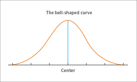
Figure 1. A bell-shaped curve

Let’s use an algebra test to illustrate. If a student takes the algebra test only once, the resulting score is called an observed score. Suppose then that the student repeats the same algebra test a countless number of times, all at the same time—yes, countless.

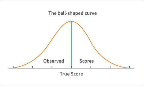
Figure 2. Distribution of observed scores

That student would have just as many observed scores as the number of times he or she has tested. Note that due to error these observed scores won’t necessarily be equal; some scores will be high and others low. If you count the number of times each of the student’s observed scores occurs and graph those counts, you’ll get a bell-shaped curve of observed scores for the student.

Most of the student’s algebra scores will  be near the center—hence the peak at the center of the bell-shaped curve—with fewer and fewer scores the further away you move from the center in either direction. This is shown in figure 2. We wouldn’t expect a student to score far below or far above what they truly know, hence the tapered ends of the curve.

The score at the center of the observed scores’ curve is what we refer to as the true score. The process of repeating the test countless times gives you the assurance that the score at the peak of the bell-shaped curve is the most common score for the student, and so it must be his or her true score. This is the score you’d expect if you could measure the student’s knowledge of algebra an endless number of times. I know what you’re thinking and you’re right: it’s impossible to test a student that many times to get their true score. We’ll come back to that in a moment.

With that distinction between an observed score and a true score, measurement error is simply defined as the difference between the two. So, if you subtracted the single true score in figure 2 from each of the observed scores, you’d have an error value for each of the observed scores. 

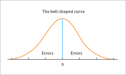
Figure 3. Distribution of errors

Observed scores that are equal to the true score have zero error, and the amount of error increases as you move away from the true score in either direction. Once again, if you  graph those error values, you’ll end up with a bell-shaped curve of errors! This time, the center is zero because the true score has no error. This is shown in figure 3.

How Do We Quantify Measurement Error?

Measurement error is reported as a number that we refer to as the standard error of measurement or SEM. From our definition of measurement error, we know that the error in the observed score shows you how far that observed score falls from the true score. Figure 3 also shows how the errors are spread out from the center, again, with the center representing a zero error value. We need a way of measuring the spread of errors from the center to the ends of the curve. So, we compute a statistic called variance. Simply put, variance determines how narrow or wide the bell-shaped curve of the errors is. In figure 4, the orange, narrow, and peaked curve is due to a smaller spread in errors compared to the flatter more stretched out blue curve. (We prefer a small spread in errors, thus the narrow orange curve.)

However, the units we use to quantify variance as a measure of spread are not directly comparable to test scores. So, we take the square root of variance to get a measure of spread that is in the same units as the scores. 

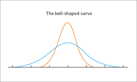
Figure 4. Large versus small variance

The square root of variance is what we call standard deviation, and the standard  deviation of the errors in figure 3 is what we call SEM. Commonly, the SEM is reported alongside a score, or it may be used to create score bands for students by adding and subtracting the SEM from a student’s score. 

The smaller the SEM, the more confidence you can have in a score. Recall that we don’t test students a countless number of times to obtain their true scores. Instead, we have statistical ways of estimating measurement error (SEM). This allows us to test a student only once, resulting in a single score along with an estimate of error in that score. It turns out that’s enough for our needs since we then know just how precise the score is by examining the associated SEM.

Measurement Error in Context

This blog post wouldn’t be complete if I didn’t tell you that there are three different testing approaches in psychometrics. The just-described method of defining SEM is based on the classical measurement approach. A different approach—called generalizability theory—divides measurement error into separate parts attributable to a specific source such as the items in the test, the test taker, the rater, etc. Yet another approach is the more recent item response theory (IRT) approach. The STAR assessments are IRT-based; each student score has a unique standard error of measurement based on the student’s achievement level. Regardless of the testing approach taken, the interpretation of SEM is the same; we just arrive at the actual values differently based on the specific psychometric approach we take.

Some Common Misconceptions

Because the SEM is a type of standard deviation, there’s a tendency to confuse the standard deviation of the observed scores in figure 2 with SEM, which is the standard deviation of the errors as in figure 3. The standard deviation of the observed scores for one student tells you how spread out the observed scores are from the true score, while the SEM tells you how much error a given observed score contains compared to the true score, which has zero error.

Another confusing issue is comparing SEM from completely different assessments and mistakenly assuming that small SEMs in one test must mean that’s a better test. This is generally not true because the size of the SEM also depends on the scale of the test scores. A test with scores ranging from 0 to 400 will likely have smaller SEMs than a test with scores ranging from 0 to 1400. For that reason, we use the published reliability level of scores to compare tests, as reliability is a standard metric that doesn’t depend on the scale of the test scores. As you’ll see below, reliability and SEM are closely related.

Finally, if you’ve searched SEM on the web, you’ve probably seen “structural equation modeling,” also known as SEM! That SEM is not the same as the SEM (standard of error of measurement) we’ve defined in this blog.

The Relationship between SEM and Reliability

As one reader wisely noted in response to my previous blog on reliability, there’s a close relationship between SEM and reliability. As one goes up, the other goes down. So, if you know that the test has highly reliable scores, you also know that the SEM is low. SEM and reliability, however, serve different purposes. The reliability value tells you how consistent the scores from a given test are from one administration to the next but doesn’t tell you how much uncertainty a student’s score contains. To evaluate the student’s performance on the test, we use the SEM associated with his or her observed score.

I hope this post has helped you learn the basics of SEM and how to use it to evaluate a student’s score. I look forward to engaging with you in the comments below and on future psychometric topics on the blog!